
Media Street have been offering a diverse range of digital services to local and international businesses for over 10 years. With a credible client portfolio and a wide knowledge of all-things-digital, we have helped businesses grow through creative website and graphic design, successful marketing campaigns and competitive hosting packages, plus much more. Take a further look into our latest news articles, learn more about our staff and how we can help your business excel with our FAQs and testimonials
Access and Manage your accounts with Media Street. To login to your client areas please select the relavent link below.
We're proud to be a full service digital agency. For a list of our services please navigate services using the menu to the left, or choose a service category below.
Alternatively you can view all of our services below:
View AllGoogle Sheets offers the same functionality as Microsoft Excel and therefore is great for analysing and working with data, making it suitable for a range of tasks. Google Sheets integrates with many tools we use in our daily work and also offers excellent collaborative functionality and remote access. In tools such as Google Ads, Google Search Console or the SEO Dashboard, it is possible to export a Google Sheet straight into your Google Drive to begin analysing or working on it.
This guide covers: basic terminology, basic functions, useful features, basic maths and automations and reports.
If you have never used Google Sheets before, here is some basic terminology to make it easier to follow the rest of this guide.
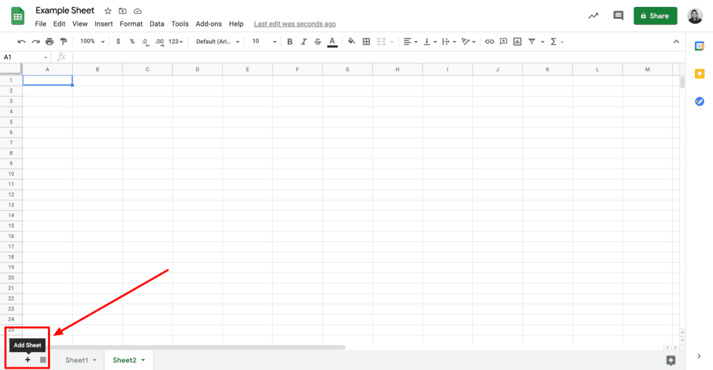
With the small plus icon in the bottom left corner, you can add new sheets. These new sheets appear at the bottom of the screen. Rename or duplicate sheets by right clicking.
Text in cells can be formatted using the tools in the top bar – i.e. bold, italics, highlight, cell outlines, etc.
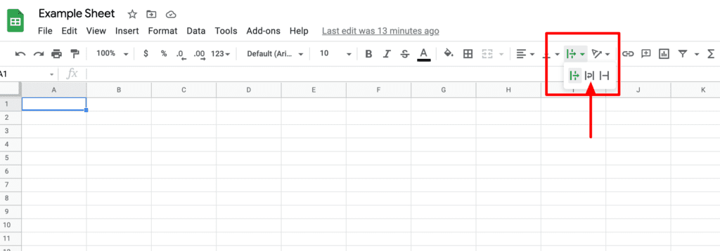
You may find you have a large amount of text in a cell and this is hard to read. To resolve this, hover over the text wrapping button and choose the middle option (as below image). This will force the text to fit within the width of the cell, making the cell taller but also so you can read it all at once.
If you are working heavily with numbers in your sheet, you may find that you have some numbers with lots of decimal places and others without. To give your sheet consistency, you can format your numbers by selecting the relevant cells, clicking the ‘Format’ menu and selecting ‘Number’. Here, you can choose how to display your numbers, and if you can’t find what you need, try looking under ‘More Formats’. This is also great for setting currency, dates or time formats.
If you need to add an extra row or column, select the row/column next to where you want the new one and right click. Select ‘Insert 1 below/above’ or ‘Insert 1 left/right’.
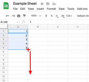
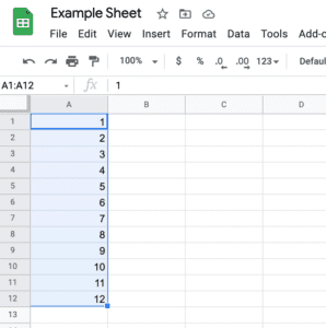
Notice a pattern to the data you’re entering? Select the data you already have, hover over the bottom right corner of the selected data and you will see a little plus cursor. Click and drag to populate the cells (see below images). This also works with numerical and alphabetical dates and also with equations.
Once you’ve exported your sheet, or added the data you require yourself, there are many features that could make your work easier. They are explained below.
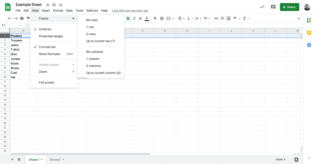
Often, when you export a sheet or when you create your own, you will make use of headings for your columns and rows. If you then need to scroll through all your data, it can get confusing as to which column contains what information. Use the Freeze tool to solve this (found under ‘View’ menu). Now, when you scroll, you will always see the frozen rows/columns.
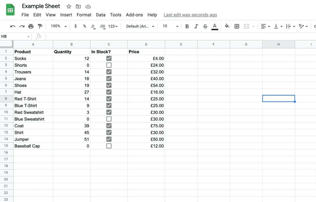
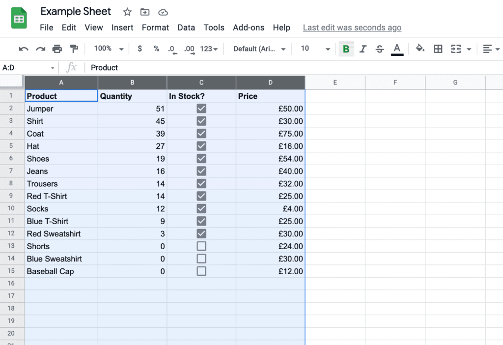
If you have a lot of rows of data or even just need to view your data in a specific order, the data sorting tool is really useful. See below image for example of some data for a clothes shop.
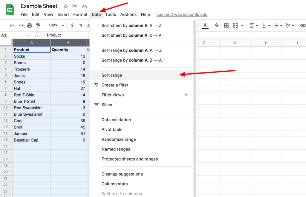
To organise this by the quantity, select the data you need to organise which in this case is all of it (Tip: if you have a lot of rows, use the A, B, C, etc. to select all data in those columns instead of scrolling to select it all), then use ‘Sort Range’ in the ‘Data’ menu.
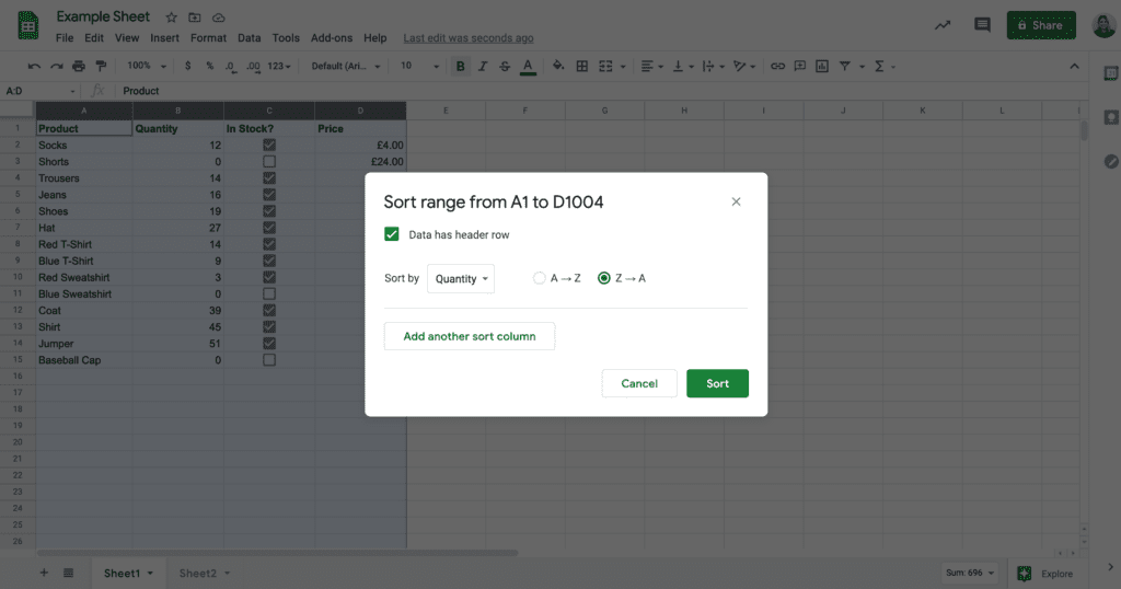
This opens a pop-up (as below image). If you tick ‘Data has a header row’, you will be able to see your headers in the ‘Sort by’ drop down. You can also select if you want to view the data lowest to highest or vice versa. For numbers, highest to lowest is ‘Z-A’.
This will re-organise the data to the below.
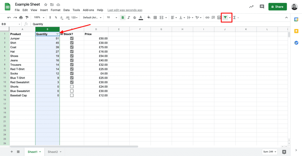
You can also use filters to organise your data. To do so, select the column you want to filter, and click the ‘Filter’ button in the top menu. This will add a filter icon at the top of the column (as shown below).
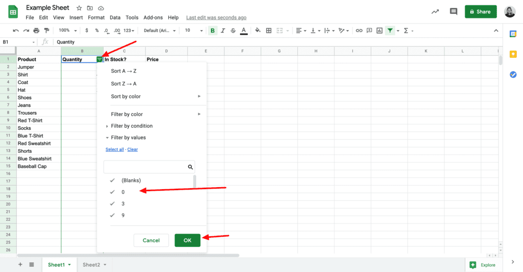
When you click the column’s filter icon, you will be able to see various options. To hide the rows where the quantity is 0, untick the ‘0’ from the list and click ‘OK’.
You can use conditional formatting to highlight cells with specific information you need. You can use conditional formatting for various purposes – a few are shown below using the same example data as above.
If you didn’t want to hide the out of stock products (by using a filter), you could just highlight them with conditional formatting.
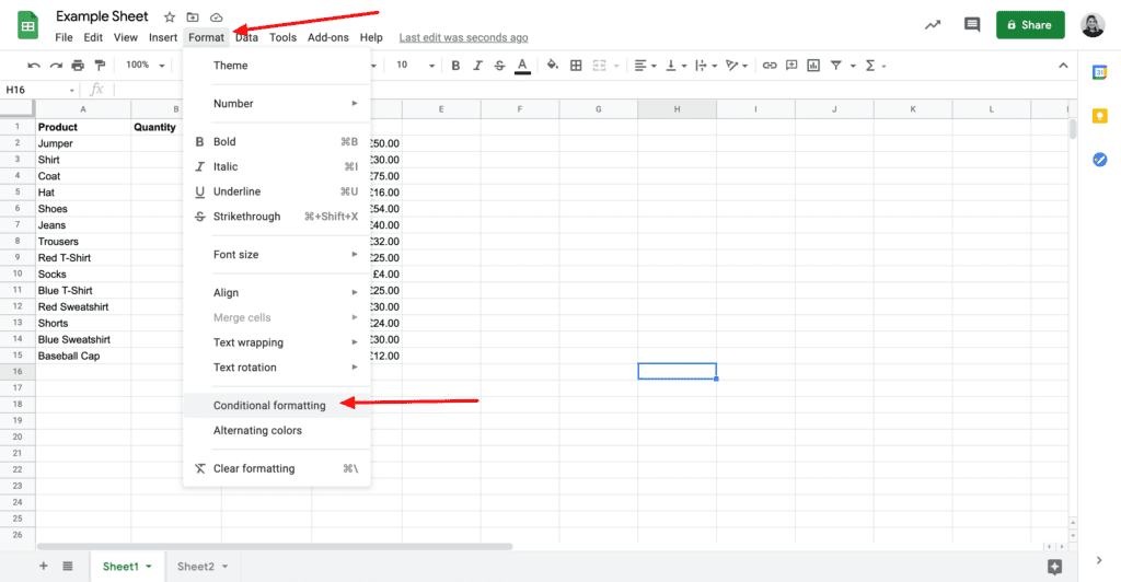
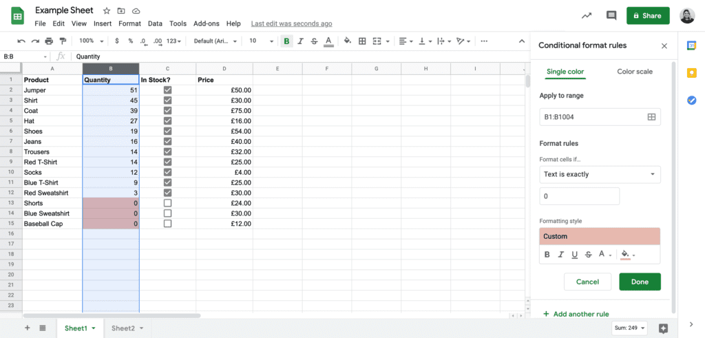
Firstly, to just highlight the cells with a ‘Quantity’ of ‘0’, select the data you want to add the formatting to, which in this case in column B, and click ‘Conditional Formatting’ under the ‘Format’ menu.
This will open a ‘rules’ sidebar where you can set the details you need. In this example, the range is column B (quantity) and we are formatting the cells if the text is exactly 0. I have then set the colour to red. Click done to save. The formatting will show automatically before you save so if you can’t see the colours change, you may need to check your rule settings.
You can then add more rules with ‘+ Add another rule’.
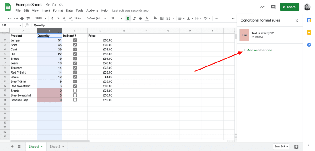
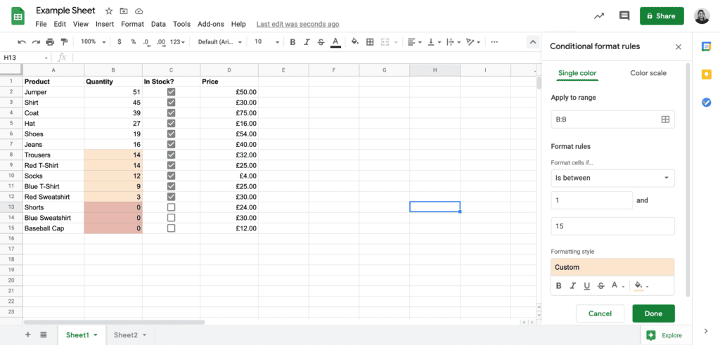
You can also highlight data between certain ranges. Add a rule in the same way but select the ‘Is between’ rule and enter your figures. In this example, we are highlighting low stock of products where the quantity is between 1 and 15 (in orange).
It is also possible to highlight whole rows. You can do this using checkboxes like in the following example.
This rule is added in a similar way to the above but this time, you should highlight all the data and go to ‘Conditional Formatting’. Now you should choose to format the cells if ‘custom formula is’ and then enter the formula: = $C1 = FALSE
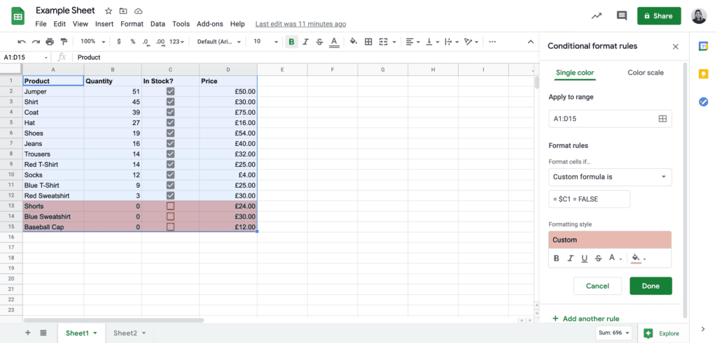
You should see the whole row of all out of stock products highlighted. Click ‘Done’ to save the rule.
Note: to highlight in stock products, change the formula to = $C1 = TRUE
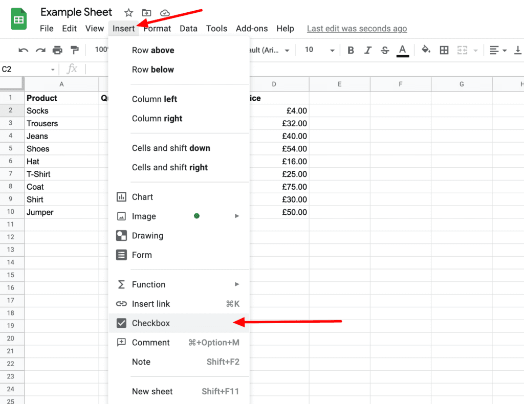
Checkboxes are great for keeping track of whether a certain task is done or if products are in stock, for example. Add them with the ‘Insert’ menu.
When working with data, there will be certain calculations you need to do to ascertain specific information. When using Google Sheets, this maths can be very easy as it can be done for you and there are a few different techniques that are particularly useful, which are shared below.
Firstly, some basic information regarding symbols needed for calculations in Google Sheets:
= Equals
+ To add
– To subtract
* To multiply
/ To divide
Adding brackets to a calculation will ensure that this part of the calculation is done first – this follows BODMAS (Brackets of Division, Multiplication, Addition, Subtraction) and will be the order for any sums you do in Google Sheets. An example of this is:
(20-2)/6*3 = 9
Equations in Google Sheets are easy to insert, there are a few ways to do this:
If you have basic maths to do, you can click the cell you want to display the answer and type: = followed by the maths you want to do (e.g. =5*3+2)
Note: you can click the cells to select their value instead of typing in the numbers manually – this is particularly useful for active sheets that keep track of stock, etc. as the equations will change dynamically with the values in the sheet.
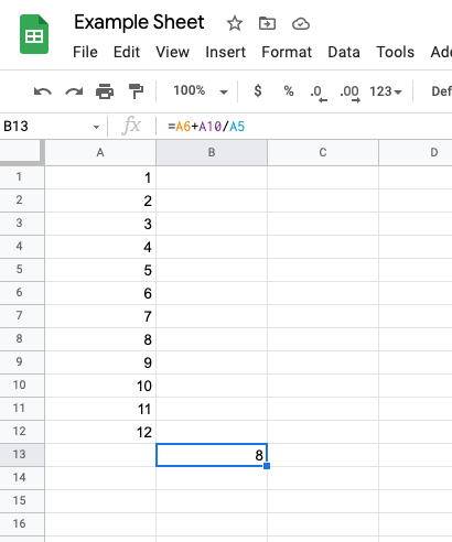
In the below example, B13=A6+A10/A5 – which is =6+10/5
Additionally, and for more complex sums, you can use the equations button in the top menu (as seen below) to choose the sum you require.
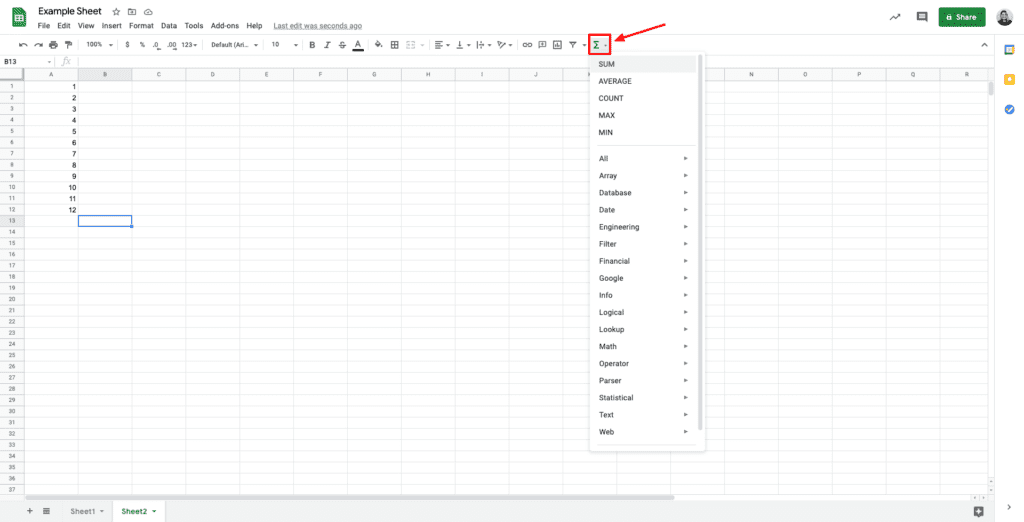
Note: if you know the equation you want to use, if you start typing in a cell =SUM (for example), you will get suggestions for the equation format which you can select and fill in the formula as needed.
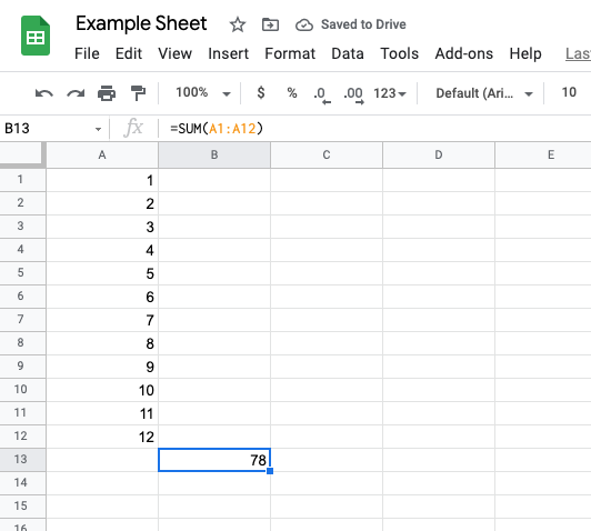
Selecting =SUM allows you to total the values of several cells at once which is great for entire rows or columns. In the below example, B13=SUM(A1:A12) which is the sum of all cells between A1 and A12 which equals 78.
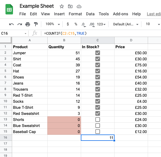
A more simple total you can do is to count the number of values you have, using =COUNT
Note: this won’t add the value of the cells, just the actual number of cells. Using the same data as above, the equations would be =COUNT(A1:12) – and the answer would be 12 as there are 12 cells with values.
You can also use =COUNTIF for checkboxes to see how many are ticked. In the below example, using =COUNTIF(C2:C15,True) shows there are 11 boxes ticked in column C.
Note: change True to False to count unticked checkboxes.
Finding the difference between two values is another common equation required. This could be useful to see how two scores have improved over time, for example.
To find the difference, you simply need to use a subtraction sum. In the below example, column C finds the difference between columns B and A. So C2=B2-A2 which is 12-1 which equals 11.
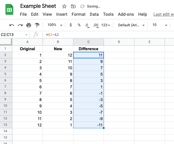
Note: you can use the select a cell and click and drag down to populate the below cells with the same formula. As demonstrated above in ‘Simplify Patterned Data Entry’.
You may be looking to find the average score or figure from your data, this is done by finding the total of the relevant cells and then dividing by the number of cells.
If you don’t know how many cells you need to divide by, you can use the count equation in your formula as with the below example.
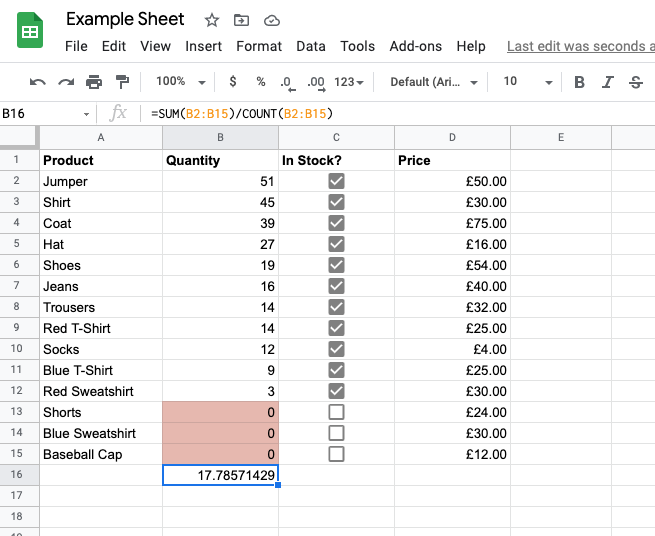
As you can see, B16=the sum of cells B2 to B15 divided by the number of cells between B2 and B15.
Note: with the above, you can then Number Format cell B16 to make it just 2 decimal places.
More simply, you can use =AVERAGE – found using the equations button.
It is likely that you will need to use percentages in your work, particularly if you are working with money as you will need to add VAT, for example.
To find the percentage of a figure (x), you can multiply x by a decimal. If finding 50%, you would multiply x by 0.5, 20% is x multiplied by 0.2, 10% is x multiplied by 0.1 and so on. If looking for 35%, this would be x multiplied by 0.35.
Example 1
In this example, x is 100
To find 40% of 100, you need to multiply 100 by 0.4 which gives you 40. This is the same as taking 100, dividing it by 100 and multiplying it by 40.
Example 2
Another example, this time x is 50 and we want to find the VAT which is always 20%
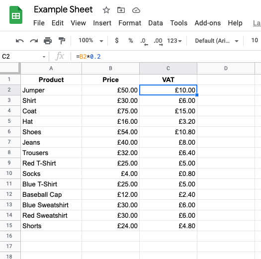
In the example above, we have used the equation =B2*0.2 which is 50 multiplied by 0.2 which equals 10. Again, this is the same as 50 divided by 100 and multiplied by 20.
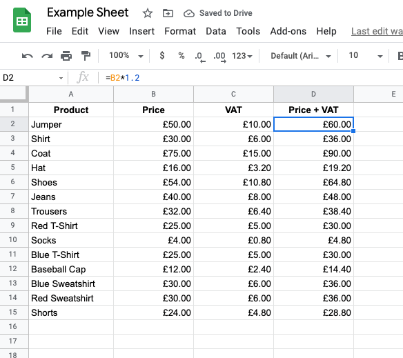
This is useful when looking to add VAT to a price. VAT is charged at 20% so this will be a case of multiplying by 0.2 and adding this figure to the original price. It is possible to use the above technique to find the VAT and add it separately but to add it in one equation, use the following formula: = x * 1.2
Example
Adding VAT to £50
When x is £50, it’s 50*1.2 which is 60 (seen below).
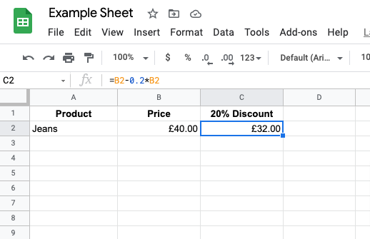
If you’re a clothing brand selling jeans with a discount of 20% off, you can work out how much you customer will pay using the following formula = x – 0.2 * x
So, if jeans you’re selling are £40, you do 40-0.2*40
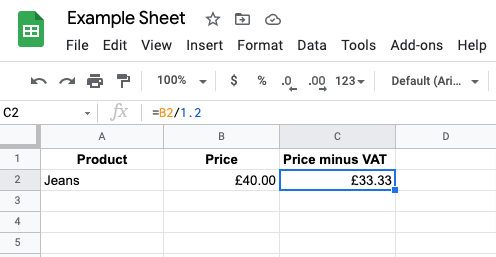
Removing VAT is not exactly the same as subtracting 20% from the customer’s price because the VAT is 20% of the original price. To remove the VAT you need to divide x by 1.2
So, the VAT off the £40 jeans is 40/1.2 which is £33.33
Say you’re looking to see the difference between two figures. The formula you need is y/x*100-100
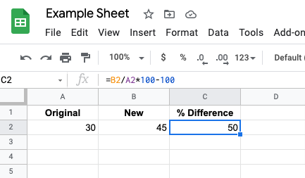
In the above example, x is 30 and y is 45
Google Sheets also integrates with a number of other programmes to provide reporting and automations. There are plugins you can use for this (speak to Charlie for more details).
Media Street uses the above functionality for Google Ads and also Forminator to get this information automatically transferred into a Google Sheet. It is possible to then set up emails from the automated reports so you can see the relevant information in your inbox every week (or however frequently is required).


 01392 914033